Code Generation

Before discussing larger compiler structures such as caching and dynamic access, it is useful to look at the small Brainfuck idioms from which Acus builds its generated code. Many of the algorithms in this chapter are simple in isolation, but together they form the vocabulary used to express higher-level operations on the tape. Moving or copying values, constructing constants or adding numbers together are all small patterns that appear repeatedly in the generated output.

This chapter is therefore not meant to be a complete catalogue of every algorithm implemented by Acus. Instead, it presents a representative selection: the basic destructive operations that make Brainfuck programming work, a few arithmetic operations, and the dynamic pointer-movement techniques that are most specific to compiling higher-level code to Brainfuck.

Clearing, Moving and Copying Values

One of the simplest useful BF idioms is destructive movement: consume one cell while adding its value somewhere else. From that, one can build addition and non-destructive copying by introducing temporary storage. Basically all other algorithms rely on repeated applications of these idioms.

Clearing Cells

A cell can be cleared simply by moving the pointer onto it and repeatedly decrementing its value until it becomes zero: [-]. If the value is known to be larger than 128, [+] may be faster at runtime, since the cell reaches zero by overflowing rather than by decrementing all the way down.

Moving Data

The contents of a cell can be moved to another by decrementing its contents while incrementing that of the other. For example, to move the contents of cell x into cell y (leaving x empty):

# MOVE(x, y)
y[-]
x[- y+ x]

Copying Data

When the contents of a cell must be copied rather than moved, we need a temporary cell. The value stored in x is then simultaneously moved into both y and the temporary scratch cell s. When the move completes, s is moved back into x to restore its value. The scratch cell s is assumed to be zero before and after the operation.

# COPY(x, y)
# Assumes s is an empty scratch cell

y[-]
x[- y+ s+ x]
s[- x+ s]

Constant Factories

Constructing known values is fundamental to creating meaningful programs. Even a simple Hello World requires the compiler to construct those characters somewhere in memory. The simplest and most naive way of setting a BF cell to some known value, e.g. n, is to concatenate n plus-commands. For example, the expression x = 20 can be compiled to:

# SET(x, 20)
x [-] ++++++++++ ++++++++++ # 23 characters + initial move sequence

Notice that the cell containing x is first cleared using [-], since we generally cannot assume that it already contains zero (even if it was freshly allocated). This particular example adds 23 characters to the generated BF output (excluding the initial move); larger values obviously produce more characters. The number of characters needed to set a cell to some constant value $c$ is simply: $$\begin{aligned} N_1(x\leftarrow c) = 3 + c + m(x) \label{eq:n1} \end{aligned}$$ where $m(x)$ is the number of move-commands necessary to reach the slot of x from the current pointer position.

To reduce code-size, we can use a scratch-cell to implement a multiplication of two smaller numbers instead. For example, instead of a series of 20 plus-commands, we can have the compiler multiply 4 and 5 to get the same result at the expense of having to use a scratch-cell s. Since scratch cells are allocated in a known-zero state and restored to zero after use, there is no need to clear s before this sequence.

# SET(x, 20)
# Assumes s is an empty scratch cell

x [-]         
s ++++ [      
  x +++++     
  s -        
]

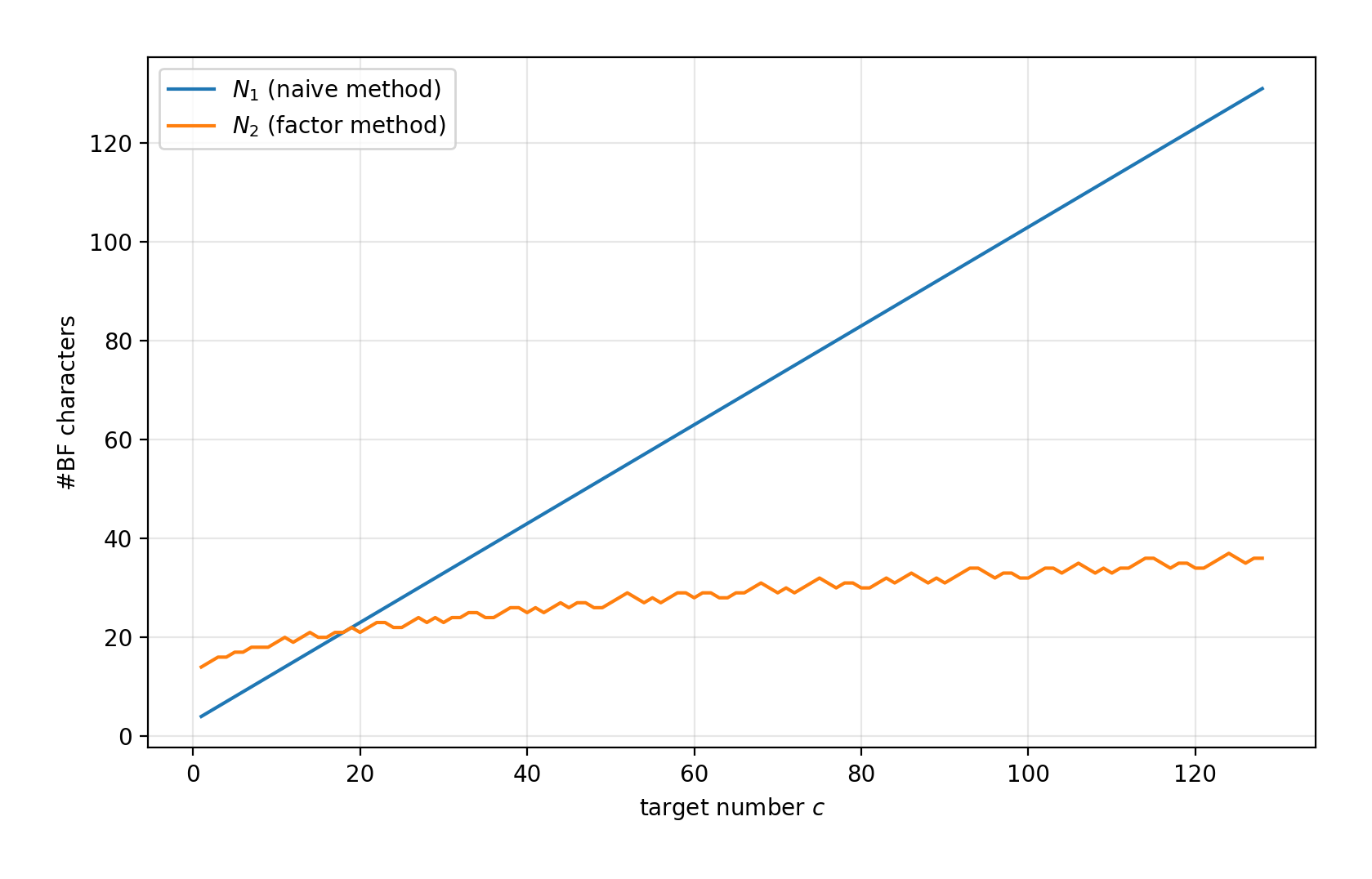
Instead of 23 characters, this algorithm adds only 15 non-movement characters to the program. In general, when $c$ can be factored into $a$ and $b$, the number of BF characters necessary to construct this value is: $$\begin{aligned} N_2(x\leftarrow ab, s) = 6 + a + b + m(x) + 3m(x, s) \label{eq:n2} \end{aligned}$$ where $m(x,s)$ is the number of move-commands necessary to move between the scratch-cell s and the target cell x. This value depends on the exact layout of a macro-cell but can be as low as 2 when the scratch-fields are right next to the value-fields. In the case where $m(x,s)=2$, the difference between both methods for this specific example is $$\begin{aligned} N_1 - N_2 &= 3 + 20 + m(x) - (6 + 4 + 5 + m(x) + 3\cdot 2) \\ &= 23 - 21 = 2. \end{aligned}$$ In this small example the saving is only two characters, while the runtime cost increases because the generated loop must be executed. Luckily the benefit from the second method increases along with the value of $c$. Acus has a precomputed table of factors for all numbers up to 128 (listed in Appendix Constant Factory Lookup Table). Larger values can be reached by decrementing using the minus command to come down from 255 rather than up from 0 (BF cells wrap around after being decremented beyond 0). Each factorization $a\times b$ is chosen in such a way that it minimizes the sum $a+b$ (and consequently the number of output characters). In some cases (e.g. when $c$ itself is prime), it is better to factor a number close to $c$ and correct for the difference after doing the multiplication. For example, the optimal way to construct the value 31 is to first construct 30, then add 1, i.e. $31 = 5\times6 + 1$ for a total cost of 24 characters (as opposed to 34) for a gain of 10 characters per construction. Figure 51 shows the number of characters generated for every constant up to 128 (the graph would be symmetric around this number when going from 129 to 255), for both methods. Acus implements both the naive and factorizing method and picks whichever produces the least amount of code.

Addition and Subtraction

Addition (8-bit)

The algorithm for addition is much like that of copying, the difference being that the target cell is never cleared in advance. When the right-hand side (rhs) of an expression of the form x += y may be destroyed, the algorithm is very short and efficient:

# DESTR_ADD_TO(x, y)
y[- x+ y]

The non-destructive version requires a scratch cell to hold a copy of the rhs operand, which can then be destroyed in the process.

# ADD_TO(x, y), preserving y
# Assumes s is an empty scratch cell

COPY(y, s)
DESTR_ADD_TO(x, s)

Addition (16-bit)

Adding 16-bit numbers together is much more involved and no BF pseudocode will be listed for this reason. Instead the higher-level pseudocode of Listing 8 illustrates the process. First, the low bytes are added together as usual. If the resulting value is less than its original value, this means that the cell has overflowed and we need to carry a 1 to the high byte. This requires multiple scratch-cells to hold temporary copies and helpers. Moreover, we need to be able to do a less-than comparison and branch on the result to carry if necessary. The implementation of this operator is discussed below in Section Less Than.

# 16-bit version of x += y
xLowBefore = low(x)
low(x) += low(y)          # normal 8-bit add
if low(x) < xLowBefore:
  high(x) += 1            # carry on overflow
high(x) += high(y)        # normal 8-bit add

Subtraction

The subtraction algorithms are symmetric to the ones for addition, where increments are substituted for decrement operations and instead of checking for overflow, we check for underflow in the 16-bit case (i.e. whether the result has grown after doing the 8-bit subtraction on the low byte).

Signed Integers

For signed integers, no special algorithms have to be used at all. Since signedness is encoded using two’s complement representation, addition and subtraction already work out of the box. Signedness becomes more important for comparisons, where the same bit pattern may represent a different ordering depending on how it is interpreted (as signed or unsigned).

Multiplication and Division

Multiplication (8-bit)

Multiplication can be implemented in terms of repeated addition, much like we already did in the constant factory optimization. To evaluate the expression x *= y, we do the following:

1. Make a copy of the operand x.

2. Clear x.

3. Repeatedly decrease y while adding the original value of x, stored in the copy, to x itself.

The steps above are the generalized version of the algorithm, which can be optimized further for edge cases where y = 0, y = 1 or even for powers of 2.

# DESTR_MUL_BY(x, y)
# Assumes s is an empty scratch cell

COPY(x, s)
x [-]
y [-
  ADD_TO(x, s)
]

Like before, this algorithm destroys the rhs operand in the process. A non-destructive version can be written in terms of the destructive version:

# MUL_BY(x, y)
# Assumes s is an empty scratch cell

COPY(y, s)
DESTR_MUL_BY(x, s)

Multiplication (16-bit)

A naive 16-bit algorithm can simply follow the exact same procedure by relying on 16-bit addition. However, this leads to a lot of additions for large factors, which can slow down the runtime significantly. Instead, we can perform a small series of 8-bit multiplications and additions to get the same result, realizing that the 16-bit number is stored as a 2-digit base-256 number. That is, every 16-bit integer $x$ can be written as $$\begin{aligned} x = x_0 + 256\cdot x_1, \end{aligned}$$ where $x_0$ and $x_1$ are the low and high bytes of $x$ respectively. Multiplication then becomes: $$\begin{aligned} z = x \times y &= (x_0 + 256x_1)(y_0 + 256y_1) \\ &= x_0y_0 + 256\cdot(x_1y_0 + x_0y_1) + 256^2\cdot(x_1y_1) \end{aligned}$$ The final term only contributes to bits beyond the lowest 16 bits, so it can be discarded when the result is stored as a 16-bit value. This means that the low and high byte of the product $z$ can be expressed as $$\begin{aligned} z_0 &= x_0 y_0 \bmod 256 \\ z_1 &= \left(x_0 y_1 + x_1 y_0 + \left\lfloor \frac{x_0 y_0}{256} \right\rfloor \right) \bmod 256 \end{aligned}$$ Therefore, the 16-bit product can be computed using three 8-bit multiplications. The low byte of the result comes from the low byte of $x_0y_0$, while the high byte receives the carry from this product together with the low bytes of the two cross-products.

p0 = low(x)  * low(y)
p1 = low(x)  * high(y)
p2 = high(x) * low(y)

low(z)  = low(p0)
high(z) = low(p1 + p2 + high(p0))

Division (8-bit and 16-bit)

Unsigned division is implemented using repeated subtraction. Given two values x and nonzero y, the goal is to compute a quotient q and remainder r such that $$\begin{aligned} x = qy + r, \qquad 0 \leq r < y. \end{aligned}$$ The simplest way to do this is to repeatedly subtract y from a running remainder until doing so would make it negative. The number of successful subtractions is the quotient, while the value left behind is the remainder.

For 8-bit unsigned values, this can be expressed by first copying the dividend into r and clearing q. Then, as long as r is greater than or equal to the divisor, the divisor is subtracted from r and q is incremented. In high-level pseudocode:

# unsigned 8-bit division: x / y
q = 0
r = x

while r >= y:
  r -= y
  q += 1

The actual BF implementation cannot test r >= y directly. Instead, this comparison is implemented using scratch cells: temporary copies of r and y are decremented together until one of them reaches zero. If the copy of y reaches zero first or at the same time as r, the subtraction is safe and the loop may continue. If the copy of r reaches zero first, the next subtraction would underflow and the algorithm terminates. The original values must either be preserved during this test or reconstructed afterwards, which makes division considerably more expensive than addition or multiplication.

The same idea also applies to 16-bit unsigned division. The quotient is repeatedly incremented while the divisor is subtracted from a 16-bit remainder. The only difference is that the comparison and subtraction are now multi-byte operations, using the borrow and comparison mechanisms described earlier. This makes the algorithm correct but relatively slow for large quotients, since the number of loop iterations is proportional to the resulting quotient.

The generated implementation handles a zero divisor separately according to the rules in Section Division by Zero.

Signed Multiplication and Division

Signed multiplication and division are implemented as thin layers around the corresponding unsigned algorithms. First, the sign bit of the left-hand side is inspected. If it is set, the value is negated in place and a temporary flag is set to indicate that the final result should be negative. The right-hand side is copied into temporary storage before its sign is inspected, so the original divisor or multiplier does not have to be modified. If this copy is negative, it is negated as well and the result-sign flag is toggled. At this point, both operands have been converted to positive values, while the temporary flag records whether the original operands had opposite signs.

The actual multiplication or division can then be performed using the unsigned algorithm. After this operation has completed, the result-sign flag is checked. If it is set, the result is negated back into two’s complement form. This approach avoids having to implement separate signed versions of the core multiplication and division algorithms; signedness is handled only by pre-processing the operands and post-processing the result.

When division also produces a remainder, Acus follows the same convention as C++ integer division: the quotient is truncated toward zero and the remainder has the same sign as the dividend. In other words, for x / y and x % y, the generated code preserves the relation $$\begin{aligned} x = (x / y)\cdot y + (x\%y), \end{aligned}$$ where x % y follows the sign of x. This convention was chosen because it is familiar from C++ and maps naturally onto the implementation: expressions evaluated at compile-time (constant-folding) using the C++ % operator will therefore produce the same result as the runtime.

Division by Zero

To deal with division by zero, Acus will simply fill the result with the maximum value allowed by the width of the type: 255 for u8 or 65535 for u16 unsigned integers. For signed integers, the same bit-representation will be used, resulting in (a somewhat confusing) value of -1. The exception to this rule is when the numerator is 0 as well, in which case the result will become 0. Modulo operations where the denominator is 0 will always result in a value of 0.

Boolean Operations

All of the usual logic and comparison operators have been implemented in Acus, which allow the programmer to build complex logical expressions. Some of these logical building blocks will be explained below.

Conversion to Bool

The simplest boolean conversion is one where an integer is transformed into either a 0 or 1, depending on its truth-value (any non-zero is considered true). To accomplish this, the value of the operand x is moved into a scratch cell, leaving x empty. We then branch off the value of s: if non-zero, x is set back to 1. If the conditional block is not entered, x remains 0.

# BOOL(x)
# Assumes s is an empty scratch cell

MOVE(x, s)
s [[-] x+ s]

Logical Not

The not-operator does the exact opposite of a boolean conversion. It transforms its operand into 1 when its value equals 0 and vice versa for any non-zero values. The algorithm is almost identical to that of BOOL(x): instead of setting x to 0 and incrementing it in the loop-block, we set it to 1 and decrement it inside the loop.

# NOT(x)
# Assumes s is an empty scratch cell

MOVE(x, s)
x +
s [[-] x- s]

Logical And

The AND operator is implemented using a nested BF-loop block. The operands are used to decide if those blocks should be entered. The result is then set in the inner loop, which can only be reached if both operands evaluate to true.

# DESTR_AND(x, y)
# Assumes s is an empty scratch cell

MOVE(x, s)
s [[-]
  y [[-] x+ y]
  s
]

Note that the algorithm above destroys the contents of y and replaces the original value of x by the result of the operation. A non-destructive version can be implemented simply by letting the destructive version operate on copies of the operands.

Logical Or

If we compare the logical AND algorithm to two switches wired in series, where current can only flow if both switches are turned on, the OR algorithm is its parallel counterpart. Each of the operands guards a loop and if either one of them is entered, the result is set to true.

# DESTR_OR(x, y)
# Assumes s is an empty scratch cell

MOVE(x, s)
s [[-]
  x+
  s
]
y [[-]
  x[-]+
  y
]

Again, this algorithm destroys the rhs of the expression but this is easily managed by operating on a copy if necessary. Note as well that in the second loop, x has to be reduced to 0 first in case the first branch was entered as well (a short-circuiting algorithm would only increase the complexity and runtime rather than cutting down on it).

Equality

In testing for equality, we rely on the fact that $x-y=0$ when $x=y$ to implement a routine that calculates NOT(x - y).

# EQ(x, y)

SUB_FROM(x, y)
NOT(x)

Less Than

This operator was already used before in the implementation of 16-bit addition, to determine the value of the carry-bit. It is implemented by reducing both of its operands simultaneously, until either one of them reaches zero. If the rhs is still non-zero when this happens, the lhs must have been the smaller of the two. This turns out to be a pretty tedious algorithm when expressed in BF, so instead it is presented in pseudocode below. Other comparison operators are implemented similarly.

# LT(x, y)

while x AND y:
  --x
  --y

x = NOT(y)

Signed Comparisons

Comparisons on signed integers cannot use the unsigned implementations discussed before. Instead, the exact form of the algorithm depends on the sign bits of both arguments. A runtime check has to be done to determine which one of four branches must be taken. For example, for the less-than operator, if its operands are both signed:

1. If both are nonnegative, use the unsigned algorithm.

2. If the lhs is negative and the rhs is positive (or zero), return 1 immediately.

3. If the lhs is nonnegative and the rhs is negative, return 0 immediately.

4. If both are negative, use the unsigned greater-than algorithm on their absolute values.

This requires an algorithm to evaluate the sign of an integer and one to take its absolute value. To get the sign bit of an 8-bit value $x$ (1 if negative, 0 otherwise), we simply compute the result of $x >= 128$ (using the unsigned greater-equal operator). Values with bit patterns identical to unsigned values from 128 on are interpreted as negative numbers (i.e. have their highest bit set) in two’s complement representation.

To calculate the absolute value of a signed integer, its sign bit is first calculated. If not set, the value can remain unmodified since it is already positive. If the sign bit is set, it can be negated simply by subtracting it from 0.

# ABS(x)
# Assumes s to be an empty scratch-cell

if SIGN_BIT(x):
  # x = 0 - x
  SUB_FROM(s, x)
  MOVE(s, x)

Pointer Movement

BF has no random memory access instruction; the only way to reach a cell is to move the data-pointer (simply referred to as the pointer from now on) step by step, which requires the compiler to keep track of the pointer at all times. This poses a challenge for situations where the pointer has to move dynamically, i.e. to tape-locations not known at compile-time. This occurs for example when dereferencing pointers or when interacting with runtime indices into arrays.

Static Pointer Movement

In most scenarios, when the source and destination locations are known at compile time, pointer movement is straightforward: emit the required number of < or > commands. This is the common case for local slot operations within a frame, where the compiler can keep track of the current pointer position relative to the frame origin.

Dynamic Pointer Movement

The most interesting pointer-movement algorithms are the ones where the target is not known until runtime. Examples include array access by a runtime index and pointer dereferencing. These algorithms rely on metadata stored in macro-cells: markers, counters and payload fields are used so that the BF pointer can search through structured tape data and stop at the correct logical cell. We can distinguish between two different classes of dynamic pointer movement: marker-based and offset-based moves. In marker-based moves, the pointer moves along the tape until it hits some pre-set marker. In offset-based moves, the offset is stored in the payload cells and dragged along with the pointer while being reduced; when the payload becomes zero, the destination has been reached.

Marker-Based

This method relies on a marker-field, the FrameMarker or SeekMarker, being set beforehand. We can then move the pointer into the corresponding field of the current cell and move in some direction until the marker is hit.

# SEEK_LEFT()
# Assumes s to be an empty scratch-field

COPY(SeekMarker, s)
NOT(s)
s [[-]
  <<<<<<<<<            # skip to left-adjacent macro-cell
  COPY(SeekMarker, s)
  NOT(s)
  s
]

Because the pointer ends up at some unknown location, we commonly set another marker that can be used to bring the pointer back afterwards.

Offset-Based

The second class of dynamic pointer movement relies on a runtime value representing the offset being stored on the tape itself. For example, in the expression x[i], i is a variable stored on the tape that contains the element index with respect to the start of the array x. This index is converted into a macro-cell offset based on the size of the element type. To reach a specific offset, the pointer is moved to the start of the array (known at compile-time) and the offset-value is copied or moved into its payload-fields (a single one for 8-bit values and both of them for 16-bit values). The pointer is then moved to the right while the payload is moved along and decremented. When the payload hits zero, the required offset has been reached.

# TO_OFFSET(b, i)
# b = base address
# i = macro-cell offset wrt base

COPY(i, b.payload)
b.payload [-
  MOVE(b.payload, 9)    # move payload one macro-cell to the right
  >>>>>>>>>             # follow with data-pointer
]
# Pointer now points at the (empty) payload field of the target-element.

Note that, depending on the element-type of the array, the index does not always equal the actual offset in terms of the number of macro-cells. Some preprocessing needs to be done on arrays of type T when sizeof(T) is larger than 1, by multiplying the index by that size to get the actual offset.

Payload Transport

Dynamic writes are harder than dynamic reads because data has to be carried to a location that is not statically known. Acus solves this by moving values through designated payload fields. The payload travels along with the dynamic traversal and is deposited when the target macro-cell is found.

For marker-based movements, the payload can simply be moved along with the pointer because the payload fields are not used to perform the move itself. For offset-based movements, the payload fields already serve the purpose of containing the offset itself and cannot be used to transport the new value. Instead, the usual offset-based method described in Section Offset-Based is used to find the element, where a marker is planted. Then, the marker-based method is used to move the payload to that position and overwrite its value field(s).